Matrice de covariance

Apprendre encore plus Cet article peut être trop technique pour que la plupart des lecteurs le comprennent . ( janvier 2022 )Aidez -nous à l’améliorer pour le rendre compréhensible aux non-experts , sans supprimer les détails techniques. (Découvrez comment et quand supprimer ce modèle de message)

En théorie des probabilités et en statistiques , une matrice de covariance (également appelée matrice d’ auto-covariance , matrice de dispersion , matrice de variance ou matrice variance-covariance ) est une matrice carrée donnant la covariance entre chaque paire d’éléments d’un Vecteur aléatoire donné . Toute matrice de covariance est symétrique et semi-définie positive et sa diagonale principale contient des variances (c’est-à-dire la covariance de chaque élément avec lui-même).

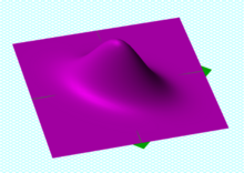Une fonction de densité de probabilité gaussienne bivariée centrée sur (0, 0), avec une matrice de covariance donnée par [ 1 0,5 0,5 1 ] {displaystyle {begin{bmatrix}1&0.5\0.5&1end{bmatrix}}} Échantillonnez des points à partir d’une Distribution gaussienne bivariée avec un écart type de 3 dans le sens approximatif inférieur gauche-supérieur droit et de 1 dans le sens orthogonal. Étant donné que les composantes x et y co-varient, les variances de X {style d’affichage x} et y {displaystyle y} ne décrit pas complètement la distribution. UN 2 × 2 {displaystyle 2fois 2} une matrice de covariance est nécessaire ; les sens des flèches correspondent aux vecteurs propres de cette matrice de covariance et leurs longueurs aux racines carrées des Valeurs propres .

Intuitivement, la matrice de covariance généralise la notion de variance à plusieurs dimensions. Par exemple, la variation d’une collection de points aléatoires dans un espace à deux dimensions ne peut pas être entièrement caractérisée par un seul nombre, pas plus que les variances dans le X {style d’affichage x} et y {displaystyle y} les instructions contiennent toutes les informations nécessaires ; un 2 × 2 {displaystyle 2fois 2} matrice serait nécessaire pour caractériser pleinement la variation bidimensionnelle.

La matrice de covariance d’un Vecteur aléatoire X {displaystyle mathbf {X} } est généralement désigné par K X X {displaystyle operatorname {K} _{mathbf {X} mathbf {X} }} ou alors Σ {displaystyle Sigma} .

Définition

Tout au long de cet article, en gras sans indice X {displaystyle mathbf {X} } et Oui {displaystyle mathbf {Y}} sont utilisés pour désigner des vecteurs aléatoires et des indices non gras X je {displaystyle X_{i}} et Oui je {displaystyle Y_{i}} sont utilisés pour désigner des variables aléatoires scalaires.

Si les entrées du Vecteur colonne

X = ( X 1 , X 2 , . . . , X n ) T {displaystyle mathbf {X} =(X_{1},X_{2},…,X_{n})^{mathrm {T} }}

sont des variables aléatoires , chacune avec une variance finie et une valeur attendue , alors la matrice de covariance K X X {displaystyle operatorname {K} _{mathbf {X} mathbf {X} }} est la matrice dont ( i , j ) {displaystyle (i,j)} entrée est la covariance ^{[1] : p. 177}

K X i X j = cov ⁡ [ X i , X j ] = E ⁡ [ ( X i − E ⁡ [ X i ] ) ( X j − E ⁡ [ X j ] ) ] {displaystyle operatorname {K} _{X_{i}X_{j}}=operatorname {cov} [X_{i},X_{j}]=operatorname {E} [(X_{i}- nomopérateur {E} [X_{i}])(X_{j}-nomopérateur {E} [X_{j}])]}

où l’opérateur E { style d’affichage nom de l’opérateur {E} } désigne la valeur attendue (moyenne) de son argument.

Nomenclatures et notations contradictoires

Les nomenclatures diffèrent. Certains statisticiens, à la suite du probabiliste William Feller dans son livre en deux volumes An Introduction to Probability Theory and Its Applications , ^[2] appellent la matrice K X X {displaystyle operatorname {K} _{mathbf {X} mathbf {X} }} la variance du Vecteur aléatoire X {displaystyle mathbf {X} } , car c’est la généralisation naturelle aux dimensions supérieures de la variance unidimensionnelle. D’autres l’appellent la matrice de covariance , car c’est la matrice des covariances entre les composantes scalaires du vecteur X {displaystyle mathbf {X} } .

var ⁡ ( X ) = cov ⁡ ( X ) = E ⁡ [ ( X − E ⁡ [ X ] ) ( X − E ⁡ [ X ] ) T ] . {displaystyle operatorname {var} (mathbf {X} )=operatorname {cov} (mathbf {X} )=operatorname {E} left[(mathbf {X} -operatorname {E} [ mathbf {X} ])(mathbf {X} -nomopérateur {E} [mathbf {X} ])^{rm {T}}right].}

Les deux formes sont assez standard et il n’y a pas d’ambiguïté entre elles. La matrice K X X {displaystyle operatorname {K} _{mathbf {X} mathbf {X} }} est aussi souvent appelée matrice de variance-covariance , puisque les termes diagonaux sont en fait des variances.

Par comparaison, la notation de la matrice de covariance croisée entre deux vecteurs est

cov ⁡ ( X , Y ) = K X Y = E ⁡ [ ( X − E ⁡ [ X ] ) ( Y − E ⁡ [ Y ] ) T ] . {displaystyle operatorname {cov} (mathbf {X} ,mathbf {Y} )=operatorname {K} _{mathbf {X} mathbf {Y} }=operatorname {E} left[( mathbf {X} -nomopérateur {E} [mathbf {X} ])(mathbf {Y} -nomopérateur {E} [mathbf {Y} ])^{rm {T}}right] .}

Propriétés

Relation avec la Matrice d’autocorrélation

La matrice d’auto-covariance K X X {displaystyle operatorname {K} _{mathbf {X} mathbf {X} }} est lié à la Matrice d’autocorrélation R X X {displaystyle operatorname {R} _{mathbf {X} mathbf {X} }} par

K X X = E ⁡ [ ( X − E ⁡ [ X ] ) ( X − E ⁡ [ X ] ) T ] = R X X − E ⁡ [ X ] E ⁡ [ X ] T {displaystyle operatorname {K} _{mathbf {X} mathbf {X} }=operatorname {E} [(mathbf {X} -operatorname {E} [mathbf {X} ])( mathbf {X} -nomopérateur {E} [mathbf {X} ])^{rm {T}}]=nomopérateur{R} _{mathbf {X} mathbf {X} }-nomopérateur { E} [mathbf {X} ]nomopérateur {E} [mathbf {X} ]^{rm {T}}}

où la Matrice d’autocorrélation est définie comme R X X = E ⁡ [ X X T ] {displaystyle operatorname {R} _{mathbf {X} mathbf {X} }=operatorname {E} [mathbf {X} mathbf {X} ^{rm {T}}]} .

Relation avec la Matrice de corrélation

Une entité étroitement liée à la matrice de covariance est la matrice des coefficients de corrélation produit-moment de Pearson entre chacune des variables aléatoires du Vecteur aléatoire. X {displaystyle mathbf {X} } , qui peut s’écrire

corr ⁡ ( X ) = ( diag ⁡ ( K X X ) ) − 1 2 K X X ( diag ⁡ ( K X X ) ) − 1 2 , {displaystyle operatorname {corr} (mathbf {X} )={big (}operatorname {diag} (operatorname {K} _{mathbf {X} mathbf {X} }){big) }^{-{frac {1}{2}}},operatorname {K} _{mathbf {X} mathbf {X} },{big (}operatorname {diag} (operatorname {K} _{mathbf {X} mathbf {X} }){big )}^{-{frac {1}{2}}},}

où diag ⁡ ( K X X ) {displaystyle operatorname {diag} (operatorname {K} _{mathbf {X} mathbf {X} })} est la matrice des éléments diagonaux de K X X {displaystyle operatorname {K} _{mathbf {X} mathbf {X} }} (c’est-à-dire une matrice diagonale des variances de X i {displaystyle X_{i}} pour i = 1 , … , n {displaystyle i=1,dots ,n} ).

De manière équivalente, la Matrice de corrélation peut être vue comme la matrice de covariance des variables aléatoires standardisées X i / σ ( X i ) {displaystyle X_{i}/sigma (X_{i})} pour i = 1 , … , n {displaystyle i=1,dots ,n} .

corr ⁡ ( X ) = [ 1 E ⁡ [ ( X 1 − μ 1 ) ( X 2 − μ 2 ) ] σ ( X 1 ) σ ( X 2 ) ⋯ E ⁡ [ ( X 1 − μ 1 ) ( X n − μ n ) ] σ ( X 1 ) σ ( X n ) E ⁡ [ ( X 2 − μ 2 ) ( X 1 − μ 1 ) ] σ ( X 2 ) σ ( X 1 ) 1 ⋯ E ⁡ [ ( X 2 − μ 2 ) ( X n − μ n ) ] σ ( X 2 ) σ ( X n ) ⋮ ⋮ ⋱ ⋮ E ⁡ [ ( X n − μ n ) ( X 1 − μ 1 ) ] σ ( X n ) σ ( X 1 ) E ⁡ [ ( X n − μ n ) ( X 2 − μ 2 ) ] σ ( X n ) σ ( X 2 ) ⋯ 1 ] . {displaystyle operatorname {corr} (mathbf {X} )={begin{bmatrix}1&{frac {operatorname {E} [(X_{1}-mu _{1})(X_{2}-mu _{2})]}{sigma (X_{1})sigma (X_{2})}}&cdots &{frac {operatorname {E} [(X_{1}-mu _{1})(X_{n}-mu _{n})]}{sigma (X_{1})sigma (X_{n})}}\\{frac {operatorname {E} [(X_{2}-mu _{2})(X_{1}-mu _{1})]}{sigma (X_{2})sigma (X_{1})}}&1&cdots &{frac {operatorname {E} [(X_{2}-mu _{2})(X_{n}-mu _{n})]}{sigma (X_{2})sigma (X_{n})}}\\vdots &vdots &ddots &vdots \\{frac {operatorname {E} [(X_{n}-mu _{n})(X_{1}-mu _{1})]}{sigma (X_{n})sigma (X_{1})}}&{frac {operatorname {E} [(X_{n}-mu _{n})(X_{2}-mu _{2})]}{sigma (X_{n})sigma (X_{2})}}&cdots &1end{bmatrix}}.}

Chaque élément sur la diagonale principale d’une Matrice de corrélation est la corrélation d’une variable aléatoire avec elle-même, qui est toujours égale à 1. Chaque Élément hors diagonale est compris entre -1 et +1 inclus.

Inverse de la matrice de covariance

L’inverse de cette matrice, K X X − 1 {displaystyle operatorname {K} _{mathbf {X} mathbf {X} }^{-1}} , si elle existe, est la matrice de covariance inverse, également appelée matrice de concentration ou matrice de précision . ^[3]

Propriétés de base

Pour K X X = var ⁡ ( X ) = E ⁡ [ ( X − E ⁡ [ X ] ) ( X − E ⁡ [ X ] ) T ] {displaystyle operatorname {K} _{mathbf {X} mathbf {X} }=operatorname {var} (mathbf {X} )=operatorname {E} left[left(mathbf {X } -nomopérateur {E} [mathbf {X} ]right)left(mathbf {X} -nomopérateur {E} [mathbf {X} ]right)^{rm {T}} à droite]} et μ X = E ⁡ [ X ] {displaystyle mathbf {mu _{X}} =operatorname {E} [{textbf {X}}]} , où X = ( X 1 , … , X n ) T {displaystyle mathbf {X} =(X_{1},ldots ,X_{n})^{rm {T}}} est un n {displaystyle n} -variable aléatoire dimensionnelle, les propriétés de base suivantes s’appliquent : ^[4]

1. K X X = E ⁡ ( X X T ) − μ X μ X T {displaystyle operatorname {K} _{mathbf {X} mathbf {X} }=operatorname {E} (mathbf {XX^{rm {T}}})-mathbf {mu _{ X}} mathbf {mu _{X}} ^{rm {T}}}
2. K X X {displaystyle operatorname {K} _{mathbf {X} mathbf {X} },} est semi-défini positif , c’est-à-dire a T K X X ⁡ a ≥ 0 for all a ∈ R n {displaystyle mathbf {a} ^{T}operatorname {K} _{mathbf {X} mathbf {X} }mathbf {a} geq 0quad {text{for all}}mathbf {a} in mathbb {R} ^{n}}
3. K X X {displaystyle operatorname {K} _{mathbf {X} mathbf {X} },} est symétrique , c’est-à-dire K X X T = K X X {displaystyle operatorname {K} _{mathbf {X} mathbf {X} }^{rm {T}}=operatorname {K} _{mathbf {X} mathbf {X} }}
4. Pour toute constante (c’est-à-dire non aléatoire) m × n {displaystyle mfois n} matrice A {displaystyle mathbf {A}} et constante m × 1 {displaystyle mfois 1} vecteur a {displaystyle mathbf {a} } , on a var ⁡ ( A X + a ) = A var ⁡ ( X ) A T {displaystyle operatorname {var} (mathbf {AX} +mathbf {a} )=mathbf {A} ,operatorname {var} (mathbf {X} ),mathbf {A} ^{ rm{T}}}
5. Si Y {displaystyle mathbf {Y}} est un autre Vecteur aléatoire de même dimension que X {displaystyle mathbf {X} } , alors var ⁡ ( X + Y ) = var ⁡ ( X ) + cov ⁡ ( X , Y ) + cov ⁡ ( Y , X ) + var ⁡ ( Y ) {displaystyle operatorname {var} (mathbf {X} +mathbf {Y} )=operatorname {var} (mathbf {X} )+operatorname {cov} (mathbf {X} ,mathbf { Y} )+nomopérateur {cov} (mathbf {Y} ,mathbf {X} )+nomopérateur {var} (mathbf {Y} )} où cov ⁡ ( X , Y ) {displaystyle operatorname {cov} (mathbf {X} ,mathbf {Y} )} est la matrice de covariance croisée de X {displaystyle mathbf {X} } et Y {displaystyle mathbf {Y}} .

Matrices de blocs

La moyenne commune μ {displaystyle mathbf {mu } } et matrice de covariance conjointe Σ {displaystyle mathbf {Sigma } } de X {displaystyle mathbf {X} } et Y {displaystyle mathbf {Y}} peut être écrit sous forme de bloc

μ = [ μ X μ Y ] , Σ = [ K X X K X Y K Y X K Y Y ] {displaystyle mathbf {mu } ={begin{bmatrix}mathbf {mu _{X}} \mathbf {mu _{Y}} end{bmatrix}},qquad mathbf { Sigma } ={begin{bmatrix}nomopérateur{K} _{mathbf {XX} }&nomopérateur{K} _{mathbf {XY} }\nomopérateur{K} _{mathbf {YX } }&nomopérateur {K} _{mathbf {YY} }end{bmatrix}}}

où K X X = var ⁡ ( X ) {displaystyle operatorname {K} _{mathbf {XX} }=operatorname {var} (mathbf {X} )} , K Y Y = var ⁡ ( Y ) {displaystyle operatorname {K} _{mathbf {YY} }=operatorname {var} (mathbf {Y} )} et K X Y = K Y X T = cov ⁡ ( X , Y ) {displaystyle operatorname {K} _{mathbf {XY} }=operatorname {K} _{mathbf {YX} }^{rm {T}}=operatorname {cov} (mathbf {X} ,mathbf {Y} )} .

K X X {displaystyle operatorname {K} _{mathbf {XX} }} et K Y Y {displaystyle operatorname {K} _{mathbf {YY} }} peuvent être identifiées comme les matrices de variance des distributions marginales pour X {displaystyle mathbf {X} } et Y {displaystyle mathbf {Y}} respectivement.

Si X {displaystyle mathbf {X} } et Y {displaystyle mathbf {Y}} sont conjointement normalement distribués ,

X , Y ∼ N ( μ , Σ ) , {displaystyle mathbf {X} ,mathbf {Y} sim {mathcal {N}}(mathbf {mu } ,operatorname {mathbf {Sigma} } ),}

alors la Distribution conditionnelle pour Y {displaystyle mathbf {Y}} donné X {displaystyle mathbf {X} } est donné par

Y ∣ X ∼ N ( μ Y | X , K Y | X ) , {displaystyle mathbf {Y} mid mathbf {X} sim {mathcal {N}}(mathbf {mu _{Y|X}} ,operatorname {K} _{mathbf {Y |X} }),} ^[5]

défini par Moyenne conditionnelle

μ Y | X = μ Y + K Y X ⁡ K X X − 1 ⁡ ( X − μ X ) {displaystyle mathbf {mu _{Y|X}} =mathbf {mu _{Y}} +operatorname {K} _{mathbf {YX} }operatorname {K} _{mathbf { XX} }^{-1}left(mathbf {X} -mathbf {mu _{X}} right)}

et variance conditionnelle

K Y | X = K Y Y − K Y X ⁡ K X X − 1 ⁡ K X Y . {displaystyle operatorname {K} _{mathbf {Y|X} }=operatorname {K} _{mathbf {YY} }-operatorname {K} _{mathbf {YX} }operatorname {K} } _{mathbf {XX} }^{-1}nomopérateur {K} _{mathbf {XY} }.}

La matrice K Y X ⁡ K X X − 1 {displaystyle operatorname {K} _{mathbf {YX} }operatorname {K} _{mathbf {XX} }^{-1}} est connue comme la matrice des coefficients de régression , tandis qu’en algèbre linéaire K Y | X {displaystyle operatorname {K} _{mathbf {Y|X} }} est le complément de Schur de K X X {displaystyle operatorname {K} _{mathbf {XX} }} dans Σ {displaystyle mathbf {Sigma } } .

La matrice des coefficients de régression peut souvent être donnée sous forme transposée, K X X − 1 ⁡ K X Y {displaystyle operatorname {K} _{mathbf {XX} }^{-1}operatorname {K} _{mathbf {XY} }} , adapté à la post-multiplication d’un vecteur ligne de variables explicatives X T {displaystyle mathbf {X} ^{rm {T}}} plutôt que de pré-multiplier un Vecteur colonne X {displaystyle mathbf {X} } . Sous cette forme ils correspondent aux coefficients obtenus en inversant la matrice des Équations normales des moindres carrés ordinaires (OLS).

Matrice de covariance partielle

Une matrice de covariance avec tous les éléments non nuls nous indique que toutes les variables aléatoires individuelles sont interdépendantes. Cela signifie que les variables ne sont pas seulement directement corrélées, mais également corrélées indirectement via d’autres variables. Souvent, ces corrélations indirectes de mode commun sont triviales et sans intérêt. Ils peuvent être supprimés en calculant la matrice de covariance partielle, c’est-à-dire la partie de la matrice de covariance qui ne montre que la partie intéressante des corrélations.

Si deux vecteurs de variables aléatoires X {displaystyle mathbf {X} } et Y {displaystyle mathbf {Y}} sont corrélés via un autre vecteur I {displaystyle mathbf {je}} , ces dernières corrélations sont supprimées dans une matrice ^[6]

K X Y ∣ I = pcov ⁡ ( X , Y ∣ I ) = cov ⁡ ( X , Y ) − cov ⁡ ( X , I ) cov ⁡ ( I , I ) − 1 cov ⁡ ( I , Y ) . {displaystyle operatorname {K} _{mathbf {XYmid I} }=operatorname {pcov} (mathbf {X} ,mathbf {Y} mid mathbf {I} )=operatorname {cov } (mathbf {X} ,mathbf {Y} )-nomopérateur {cov} (mathbf {X} ,mathbf {I} )nomopérateur {cov} (mathbf {I} ,mathbf {I} )^{-1}nomopérateur {cov} (mathbf {I} ,mathbf {Y} ).}

La matrice de covariance partielle K X Y ∣ I {displaystyle operatorname {K} _{mathbf {XYmid I} }} est effectivement la matrice de covariance simple K X Y {displaystyle operatorname {K} _{mathbf {XY} }} comme si les variables aléatoires sans intérêt I {displaystyle mathbf {je}} ont été maintenus constants.

Matrice de covariance comme paramètre d’une distribution

Si un Vecteur colonne X {displaystyle mathbf {X} } de n {displaystyle n} variables aléatoires éventuellement corrélées est conjointement distribuée normalement , ou plus généralement distribuée elliptiquement , alors sa fonction de densité de probabilité f ⁡ ( X ) {displaystyle operatorname {f} (mathbf {X} )} peut être exprimé en termes de matrice de covariance Σ {displaystyle mathbf {Sigma } } comme suit ^[6]

f ⁡ ( X ) = ( 2 π ) − n / 2 | Σ | − 1 / 2 exp ⁡ ( − 1 2 ( X − μ ) T Σ − 1 ( X − μ ) ) , {displaystyle operatorname {f} (mathbf {X} )=(2pi )^{-n/2}|mathbf {Sigma} |^{-1/2}exp left(-{ tfrac {1}{2}}mathbf {(X-mu )^{rm {T}}Sigma ^{-1}(X-mu )} right),}

où μ = E ⁡ [ X ] {displaystyle mathbf {mu =nomopérateur {E} [X]} } et | Σ | {displaystyle |mathbf {Sigma} |} est le déterminant de Σ {displaystyle mathbf {Sigma } } .

Matrice de covariance en tant qu’opérateur linéaire

Appliquée à un vecteur, la matrice de covariance mappe une combinaison linéaire c des variables aléatoires X sur un vecteur de covariances avec ces variables : c T Σ = cov ⁡ ( c T X , X ) {displaystyle mathbf {c} ^{rm {T}}Sigma =operatorname {cov} (mathbf {c} ^{rm {T}}mathbf {X} ,mathbf {X}) } . Traitée comme une forme bilinéaire , elle donne la covariance entre les deux combinaisons linéaires : d T Σ c = cov ⁡ ( d T X , c T X ) {displaystyle mathbf {d} ^{rm {T}}Sigma mathbf {c} =operatorname {cov} (mathbf {d} ^{rm {T}}mathbf {X} , mathbf {c} ^{rm {T}}mathbf {X} )} . La variance d’une combinaison linéaire est alors c T Σ c {displaystyle mathbf {c} ^{rm {T}}Sigma mathbf {c} } , sa covariance avec elle-même.

De même, la matrice de covariance (pseudo-) inverse fournit un produit interne ⟨ c − μ | Σ + | c − μ ⟩ {displaystyle langle c-mu |Sigma ^{+}|c-mu rangle } , qui induit la distance de Mahalanobis , une mesure de “l’improbabilité” de c . ^{[ citation nécessaire ]}

Quelles matrices sont des matrices de covariance ?

De l’identité juste au-dessus, soit b {displaystyle mathbf {b} } être un ( p × 1 ) {displaystyle (pfois 1)} vecteur à valeurs réelles, alors

var ⁡ ( b T X ) = b T var ⁡ ( X ) b , {displaystyle operatorname {var} (mathbf {b} ^{rm {T}}mathbf {X} )=mathbf {b} ^{rm {T}}operatorname {var} (mathbf {X} )mathbf {b} ,,}

qui doit toujours être non négatif, puisqu’il s’agit de la variance d’une variable aléatoire à valeur réelle, donc une matrice de covariance est toujours une Matrice semi-définie positive .

L’argument ci-dessus peut être développé comme suit :

w T E ⁡ [ ( X − E ⁡ [ X ] ) ( X − E ⁡ [ X ] ) T ] w = E ⁡ [ w T ( X − E ⁡ [ X ] ) ( X − E ⁡ [ X ] ) T w ] = E ⁡ [ ( w T ( X − E ⁡ [ X ] ) ) 2 ] ≥ 0 , {displaystyle {begin{aligned}&w^{rm {T}}operatorname {E} left[(mathbf {X} -operatorname {E} [mathbf {X} ])(mathbf { X} -nomopérateur {E} [mathbf {X} ])^{rm {T}}right]w=nomopérateur{E} left[w^{rm {T}}(mathbf { X} -nomopérateur {E} [mathbf {X} ])(mathbf {X} -nomopérateur {E} [mathbf {X} ])^{rm {T}}wdroite]\ &=nomopérateur {E} {big [}{big (}w^{rm {T}}(mathbf {X} -nomopérateur {E} [mathbf {X} ]){big) }^{2}{big ]}geq 0,end{aligné}}} où la dernière inégalité découle de l’observation que w T ( X − E ⁡ [ X ] ) {displaystyle w^{rm {T}}(mathbf {X} -nomopérateur {E} [mathbf {X} ])} est un scalaire.

Inversement, toute Matrice semi-définie positive symétrique est une matrice de covariance. Pour voir cela, supposons M {displaystyle M} est un p × p {displaystyle pfois p} matrice symétrique positive-semi-définie. Du cas de dimension finie du théorème spectral , il s’ensuit que M {displaystyle M} a une racine carrée symétrique non négative , qui peut être notée M ^1/2 . Laisser X {displaystyle mathbf {X} } être n’importe lequel p × 1 {displaystyle pfois 1} colonne variable aléatoire à valeur vectorielle dont la matrice de covariance est la p × p {displaystyle pfois p} matrice d’identité. Puis

var ⁡ ( M 1 / 2 X ) = M 1 / 2 var ⁡ ( X ) M 1 / 2 = M . {displaystyle operatorname {var} (mathbf {M} ^{1/2}mathbf {X} )=mathbf {M} ^{1/2},operatorname {var} (mathbf {X} } ),mathbf {M} ^{1/2}=mathbf {M} .}

Vecteurs aléatoires complexes

La variance d’une variable aléatoire à valeur scalaire complexe avec une valeur attendue μ {displaystylemu} est classiquement défini par la Conjugaison complexe :

var ⁡ ( Z ) = E ⁡ [ ( Z − μ Z ) ( Z − μ Z ) ̄ ] , {displaystyle operatorname {var} (Z)=operatorname {E} left[(Z-mu _{Z}){overline {(Z-mu _{Z})}}right], }

où le conjugué complexe d’un nombre complexe z {displaystyle z} est noté z ̄ {displaystyle {overline {z}}} ; ainsi la variance d’une variable aléatoire complexe est un nombre réel.

Si Z = ( Z 1 , … , Z n ) T { displaystyle mathbf {Z} = (Z_ {1}, ldots, Z_ {n}) ^ { mathrm {T} }} est un Vecteur colonne de variables aléatoires à valeurs complexes, alors la transposée conjuguée Z H {displaystyle mathbf {Z} ^{mathrm {H} }} est formé à la fois par transposition et conjugaison. Dans l’expression suivante, le produit d’un vecteur avec sa transposée conjuguée donne une matrice carrée appelée matrice de covariance , comme son espérance : ^{[7] : p. 293}

K Z Z = cov ⁡ [ Z , Z ] = E ⁡ [ ( Z − μ Z ) ( Z − μ Z ) H ] {displaystyle operatorname {K} _{mathbf {Z} mathbf {Z} }=operatorname {cov} [mathbf {Z} ,mathbf {Z} ]=operatorname {E} left[( mathbf {Z} -mathbf {mu _{Z}} )(mathbf {Z} -mathbf {mu _{Z}} )^{mathrm {H} }right]} ,

La matrice ainsi obtenue sera hermitienne positive semi-définie , ^[8] avec des nombres réels dans la diagonale principale et des nombres complexes hors diagonale.

Propriétés

• La matrice de covariance est une matrice hermitienne , c’est-à-dire K Z Z H = K Z Z {displaystyle operatorname {K} _{mathbf {Z} mathbf {Z} }^{mathrm {H} }=operatorname {K} _{mathbf {Z} mathbf {Z} }} . ^{[1] : p. 179}
• Les éléments diagonaux de la matrice de covariance sont réels. ^{[1] : p. 179}

Matrice de pseudo-covariance

Pour les vecteurs aléatoires complexes, un autre type de deuxième moment central, la matrice de pseudo-covariance (également appelée matrice de relation ) est définie comme suit :

J Z Z = cov ⁡ [ Z , Z ̄ ] = E ⁡ [ ( Z − μ Z ) ( Z − μ Z ) T ] {displaystyle operatorname {J} _{mathbf {Z} mathbf {Z} }=operatorname {cov} [mathbf {Z} ,{overline {mathbf {Z} }}]=operatorname { E} left[(mathbf {Z} -mathbf {mu _{Z}} )(mathbf {Z} -mathbf {mu _{Z}} )^{mathrm {T} } à droite]}

Contrairement à la matrice de covariance définie ci-dessus, la transposition hermitienne est remplacée par la transposition dans la définition. Ses éléments diagonaux peuvent avoir des valeurs complexes ; c’est une Matrice symétrique complexe .

Estimation

Si M X {displaystyle mathbf {M} _{mathbf {X} }} et M Y {displaystyle mathbf {M} _{mathbf {Y} }} sont des matrices de données centrées de dimension p × n {displaystyle pfois n} et q × n {displaystyle qfois n} respectivement, c’est-à-dire avec n colonnes d’observations de p et q lignes de variables, dont les moyennes de ligne ont été soustraites, puis, si les moyennes de ligne ont été estimées à partir des données, des matrices de covariance d’échantillon Q X X {displaystyle mathbf {Q} _{mathbf {XX} }} et Q X Y {displaystyle mathbf {Q} _{mathbf {XY} }} peut être défini comme étant

Q X X = 1 n − 1 M X M X T , Q X Y = 1 n − 1 M X M Y T {displaystyle mathbf {Q} _{mathbf {XX} }={frac {1}{n-1}}mathbf {M} _{mathbf {X} }mathbf {M} _{ mathbf {X} }^{rm {T}},qquad mathbf {Q} _{mathbf {XY} }={frac {1}{n-1}}mathbf {M} _{ mathbf {X} }mathbf {M} _{mathbf {Y} }^{rm {T}}}

ou, si les moyennes des lignes étaient connues a priori,

Q X X = 1 n M X M X T , Q X Y = 1 n M X M Y T . {displaystyle mathbf {Q} _{mathbf {XX} }={frac {1}{n}}mathbf {M} _{mathbf {X} }mathbf {M} _{mathbf { X} }^{rm {T}},qquad mathbf {Q} _{mathbf {XY} }={frac {1}{n}}mathbf {M} _{mathbf {X} }mathbf {M} _{mathbf {Y} }^{rm {T}}.}

Ces matrices de covariance d’échantillon empiriques sont les estimateurs les plus simples et les plus souvent utilisés pour les matrices de covariance, mais d’autres estimateurs existent également, y compris des estimateurs régularisés ou de rétrécissement, qui peuvent avoir de meilleures propriétés.

Applications

La matrice de covariance est un outil utile dans de nombreux domaines différents. On peut en déduire une matrice de transformation , appelée transformation de blanchiment , qui permet de décorréler complètement les données ^{[ citation nécessaire ]} ou, d’un point de vue différent, de trouver une base optimale pour représenter les données de manière compacte ^{[ citation nécessaire ]} (voir quotient de Rayleigh pour une preuve formelle et des propriétés supplémentaires des matrices de covariance). C’est ce qu’on appelle l’analyse en composantes principales (ACP) et la Transformée de Karhunen-Loève (transformée KL).

La matrice de covariance joue un rôle clé en économie financière , en particulier dans la théorie du portefeuille et son théorème de séparation des fonds communs de placement et dans le modèle d’ évaluation des actifs financiers . La matrice des covariances entre les rendements de divers actifs est utilisée pour déterminer, sous certaines hypothèses, les montants relatifs des différents actifs que les investisseurs devraient (dans une analyse normative ) ou devraient (dans une analyse positive ) choisir de détenir dans un contexte de diversification .

Cartographie des covariances

Dans la cartographie de covariance, les valeurs des cov ⁡ ( X , Y ) {displaystyle operatorname {cov} (mathbf {X} ,mathbf {Y} )} ou alors pcov ⁡ ( X , Y ∣ I ) {displaystyle operatorname {pcov} (mathbf {X} ,mathbf {Y} mid mathbf {I} )} matrice sont tracées sous la forme d’une carte en 2 dimensions. Lorsque les vecteurs X {displaystyle mathbf {X} } et Y {displaystyle mathbf {Y}} sont des fonctions aléatoires discrètes , la carte montre les relations statistiques entre les différentes régions des fonctions aléatoires. Les régions statistiquement indépendantes des fonctions apparaissent sur la carte comme des plaines de niveau zéro, tandis que les corrélations positives ou négatives apparaissent, respectivement, comme des collines ou des vallées.

En pratique les vecteurs colonnes X , Y {displaystyle mathbf {X} ,mathbf {Y} } , et I {displaystyle mathbf {je}} sont acquises expérimentalement sous forme de rangées de n {displaystyle n} échantillons, par ex.

[ X 1 , X 2 , . . . X n ] = [ X 1 ( t 1 ) X 2 ( t 1 ) ⋯ X n ( t 1 ) X 1 ( t 2 ) X 2 ( t 2 ) ⋯ X n ( t 2 ) ⋮ ⋮ ⋱ ⋮ X 1 ( t m ) X 2 ( t m ) ⋯ X n ( t m ) ] , {displaystyle [mathbf {X} _{1},mathbf {X} _{2},…mathbf {X} _{n}]={begin{bmatrix}X_{1}(t_ {1})&X_{2}(t_{1})&cdots &X_{n}(t_{1})\\X_{1}(t_{2})&X_{2}(t_{2} )&cdots &X_{n}(t_{2})\\vdots &vdots &ddots &vdots \\X_{1}(t_{m})&X_{2}(t_{ m})&cdots &X_{n}(t_{m})end{bmatrice}},}

où X j ( t i ) {displaystyle X_{j}(t_{i})} est la i -ième valeur discrète dans l’échantillon j de la Fonction aléatoire X ( t ) {displaystyle X(t)} . Les valeurs attendues nécessaires dans la formule de covariance sont estimées à l’aide de la Moyenne de l’échantillon , par exemple

⟨ X ⟩ = 1 n ∑ j = 1 n X j {displaystyle langle mathbf {X} rangle ={frac {1}{n}}sum _{j=1}^{n}mathbf {X} _{j}}

et la matrice de covariance est estimée par la matrice de covariance d’échantillon

cov ⁡ ( X , Y ) ≈ ⟨ X Y T ⟩ − ⟨ X ⟩ ⟨ Y T ⟩ , {displaystyle operatorname {cov} (mathbf {X} ,mathbf {Y} )approx langle mathbf {XY^{rm {T}}} rangle -langle mathbf {X} rangle langle mathbf {Y} ^{rm {T}}rangle ,}

où les crochets angulaires indiquent la Moyenne de l’échantillon comme avant, sauf que la correction de Bessel doit être effectuée pour éviter les biais . En utilisant cette estimation, la matrice de covariance partielle peut être calculée comme

pcov ⁡ ( X , Y ∣ I ) = cov ⁡ ( X , Y ) − cov ⁡ ( X , I ) ( cov ⁡ ( I , I ) ∖ cov ⁡ ( I , Y ) ) , {displaystyle operatorname {pcov} (mathbf {X} ,mathbf {Y} mid mathbf {I} )=operatorname {cov} (mathbf {X} ,mathbf {Y} )-operatorname {cov} (mathbf {X} ,mathbf {I} )left(operatorname {cov} (mathbf {I} ,mathbf {I} )backslash operatorname {cov} (mathbf {I} ,mathbf {Y} )right),}

où la barre oblique inverse désigne l’ opérateur de division de matrice gauche , qui contourne l’obligation d’inverser une matrice et est disponible dans certains packages de calcul tels que Matlab . ^[9]

Figure 1 : Construction d’une carte de covariance partielle de molécules de N ₂ subissant une explosion coulombienne induite par un laser à électrons libres. ^[10] Les panneaux a et b cartographient les deux termes de la matrice de covariance, qui est présentée dans le panneau c . Le panneau d cartographie les corrélations de mode commun via les fluctuations d’intensité du laser. Le panneau e cartographie la matrice de covariance partielle qui est corrigée des fluctuations d’intensité. Panneau fmontre qu’une surcorrection de 10 % améliore la carte et rend les corrélations ion-ion clairement visibles. En raison de la conservation de la quantité de mouvement, ces corrélations apparaissent sous forme de lignes approximativement perpendiculaires à la ligne d’autocorrélation (et aux modulations périodiques qui sont provoquées par la sonnerie du détecteur).

La figure 1 illustre comment une carte de covariance partielle est construite sur un exemple d’expérience réalisée au laser à électrons libres FLASH à Hambourg. ^[10] La Fonction aléatoire X ( t ) {displaystyle X(t)} est le spectre de temps de vol des ions d’une explosion coulombienne de molécules d’azote ionisées par multiplication par une impulsion laser. Comme seules quelques centaines de molécules sont ionisées à chaque impulsion laser, les spectres monocoup sont très fluctuants. Cependant, la collecte généralement m = 10 4 {displaystyle m=10^{4}} de tels spectres, X j ( t ) {displaystyle mathbf {X} _{j}(t)} , et en les faisant la moyenne sur j {displaystyle j} produit un spectre lisse ⟨ X ( t ) ⟩ {displaystyle langle mathbf {X} (t)rangle } , qui est représenté en rouge au bas de la Fig. 1. Le spectre moyen ⟨ X ⟩ {displaystyle langle mathbf {X} rangle } révèle plusieurs ions azote sous forme de pics élargis par leur énergie cinétique, mais trouver les corrélations entre les étages d’ionisation et les impulsions ioniques nécessite de calculer une carte de covariance.

Dans l’exemple de la Fig. 1 spectres X j ( t ) {displaystyle mathbf {X} _{j}(t)} et Y j ( t ) {displaystyle mathbf {Y} _{j}(t)} sont les mêmes, sauf que la plage du temps de vol t {displaystyle t} diffère. Le panneau a montre ⟨ X Y T ⟩ {displaystyle langle mathbf {XY^{rm {T}}} rangle } , le panneau b montre ⟨ X ⟩ ⟨ Y T ⟩ {displaystyle langle mathbf {X} rangle langle mathbf {Y^{rm {T}}} rangle } et le panneau c montre leur différence, qui est cov ⁡ ( X , Y ) {displaystyle operatorname {cov} (mathbf {X} ,mathbf {Y} )} (notez un changement dans l’échelle des couleurs). Malheureusement, cette carte est submergée par des corrélations de mode commun inintéressantes induites par l’intensité du laser fluctuant d’un tir à l’autre. Pour supprimer de telles corrélations, l’intensité du laser I j {displaystyle I_{j}} est enregistré à chaque prise de vue, mis en I {displaystyle mathbf {je}} et pcov ⁡ ( X , Y ∣ I ) {displaystyle operatorname {pcov} (mathbf {X} ,mathbf {Y} mid mathbf {I} )} est calculé comme le montrent les panneaux d et e . La suppression des corrélations inintéressantes est cependant imparfaite car il existe d’autres sources de fluctuations de mode commun que l’intensité laser et en principe toutes ces sources doivent être surveillées en vecteur I {displaystyle mathbf {je}} . Pourtant, dans la pratique, il suffit souvent de surcompenser la correction de covariance partielle comme le montre le panneau f , où des corrélations intéressantes des impulsions ioniques sont maintenant clairement visibles sous forme de lignes droites centrées sur les étapes d’ionisation de l’azote atomique.

Spectroscopie infrarouge bidimensionnelle

La spectroscopie infrarouge bidimensionnelle utilise une analyse de corrélation pour obtenir des spectres 2D de la phase condensée . Il existe deux versions de cette analyse : synchrone et asynchrone . Mathématiquement, le premier est exprimé en termes de matrice de covariance d’échantillon et la technique est équivalente à la cartographie de covariance. ^[11]

Voir également

• Statistiques multivariées
• Répartition de Lewandowski-Kurowicka-Joe
• Matrice de Gramian
• Décomposition des Valeurs propres
• Forme quadratique (statistiques)
• Composants principaux

Références

1. ^ ^{un bc} Park, Kun Il (2018) ^. Principes fondamentaux des probabilités et des processus stochastiques avec des applications aux communications . Springer. ISBN 978-3-319-68074-3.
2. ^ Guillaume Feller (1971). Introduction à la théorie des probabilités et à ses applications . Wiley. ISBN 978-0-471-25709-7. Récupéré le 10 août 2012 .
3. ^ Wasserman, Larry (2004). Toutes les statistiques : un cours concis sur l’inférence statistique . ISBN 0-387-40272-1.
4. ^ Taboga, Marco (2010). “Conférences sur la théorie des probabilités et les statistiques mathématiques” .
5. ^ Eaton, Morris L. (1983). Statistiques multivariées : une approche par espace vectoriel . John Wiley et fils. p. 116–117. ISBN 0-471-02776-6.
6. ^ ^{un b} WJ Krzanowski “Principes d’Analyse Multivariée” (Oxford University Press, New York, 1988), Chap. 14.4 ; KV Mardia, JT Kent et JM Bibby “Analyse multivariée (Academic Press, Londres, 1997), Chap. 6.5.3; TW Anderson “An Introduction to Multivariate Statistical Analysis” (Wiley, New York, 2003), 3e éd., Chaps 2.5.1 et 4.3.1.
7. ^ Lapidoth, Amos (2009). Une fondation en communication numérique . La presse de l’Universite de Cambridge. ISBN 978-0-521-19395-5.
8. ^ Brookes, Mike. « Le manuel de référence de la matrice » . {{cite journal}}: Cite journal requires |journal= (help)
9. ^ LJ Frasinski “Techniques de cartographie de covariance” J. Phys. Chauve souris. Mol. Opter. Phys. 49 152004 (2016), accès libre
10. ^ ^{a b} O Kornilov, M Eckstein, M Rosenblatt, CP Schulz, K Motomura, A Rouzée, J Klei, L Foucar, M Siano, A Lübcke, F. Schapper, P Johnsson, DMP Holland, T Schlatholter, T Marchenko, S Düsterer, K Ueda, MJJ Vrakking et LJ Frasinski “Explosion coulombienne de molécules diatomiques dans des champs XUV intenses cartographiés par covariance partielle” J. Phys. Chauve souris. Mol. Opter. Phys. 46 164028 (2013), accès libre
11. ^ I Noda “Méthode de corrélation bidimensionnelle généralisée applicable à l’infrarouge, Raman et à d’autres types de spectroscopie” Appl. Spectrosc. 47 1329–36 (1993)

Lectures complémentaires

• “Matrice de covariance” , Encyclopedia of Mathematics , EMS Press , 2001 [1994]
• Weisstein, Eric W. “Matrice de covariance” . MathWorld .
• van Kampen, NG (1981). Processus stochastiques en physique et chimie . New York : Hollande du Nord. ISBN 0-444-86200-5.